Independent Study Final Project 2
Gytis Blinstrubas
6/11/17
Independent Study
Over this last spring term my independent study consisted of me learning how to code with a program called labview. This program is a vital aspect of the research I am continuing from last term. We need to use this program because when we get data from our samples we get it in two forms. When the data is taken at the Advanced Photon Source at Argonne national lab our data is in the form in an image. Currently the labview program is built to take this data and convert it to the proper graphs we need. However, we also use our in-house X-Ray Diffractometer. The data from the XRD and the APS will give us the same result except that the XRD gives us the data in the form of the image. To be able to process our data we use a program called pdfgetx2. This program is less user friendly and much older, than labview. We want to rebuild the labview program so that we can process our data faster and the same way as we do the data from the APS. The program that is used for the APS is very large and has many components. To be able to work on the program I will first need to learn the basics of labview. My first task was to learn how to install the program onto my drive so that I can work on it remotely from any computer. To complete this task, I copied the build code from a hard drive and then put the program into my F drive. I also had to make sure to include a lot of sub programs because when this large program runs it is dependent on a lot of smaller programs. After installing this program on my drive, it was also important to learn how to use the program and make sure that it works. I then had to learn how to input my data and manipulate the program so that I can do corrections and build programs myself. The first program that I built was a simple program. This program allows the user to input two numbers and then choose for the program to either add, subtract, multiply, or divide those two numbers. The program works by adding specific icons to a block diagram and then connecting the icons to create the final code which function properly. On the front diagram three boxes are displayed, where two of the boxes are for inputting the numbers and the third box shows your final answer. After creating this simple program and learning the basic skills to be able to create VI’s, I then started to learn specific code that would help me in recreating the program we use for Argonne. The first code I built was a VI that could input excel files and create a graph from those files. My first step in creating this code was inserting two read delimited icons on the block diagram. Two icons are needed since one will read the data for the X axis while one will read it for the Y. The reason why I need these icons specifically is that they are able to read 2d arrays of scalar numbers. When importing my files, they will need to be converted to comma delimited files in order for labview to read this data. Off of the read delimited file a constant needs to be added, our constant in this case is the comma since we are importing the comma delimited files. The next step I took is to insert an express VI called “Build XY Graph”. This is used since an express VI has many applications and is more user friendly than a normal VI. For our case we need this express VI because it converts our raw data into graph form. The last step is to add a xy graph icon so that our graph can be seen on the front diagram. This icon will be connected to the express VI. An example of the code can be seen below.
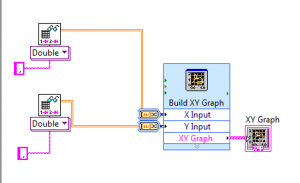
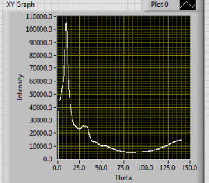
The icons and the constant can be seen to the left, where the constants are the pink boxes with a comma. With the yellow wire, each icon is either attached to the x or y input. Lastly the xy graph icon is attached to the build xy graph icon in order for the program to display the data in a graph form.. An intensity versus theta graph of an empty 2mm capillary can be seen below.
After creating a program to be able to insert text files, my next task was to create a program that could display images. The process of inserting a picture into labview is not overly complicated. The first icon that is needed is a read JPEG file. The purpose of this is that it takes the image and converts it into data that labview can read. Then connected to this icon is another icon called Draw Flattened Pixel map. This is used to create the picture. Finally, a picture icon is added. This icon takes our picture from before and displays it on the front diagram. After inserting the image, my final task was to take my image and display it on an intensity graph. With my research partner Sven Marnauzs we built a code that could accomplish this task. The first icon that was put in was a file path, this is done so that we can insert our saved image. Then the read JPEG file and the Draw Flattened Pixel map icons are inserted. After that, a picture to pix map icon is inserted and a constant is added to the icon to tell how many bits the picture is. The next icon added is an unflattened pixmap. This icon unflattens the data from the Draw Flattened Pixel map icon. The last icon added is the intensity graph, so that our image can be seen on the front panel. An example of the code can be seen below.
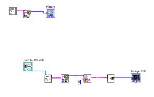
The top codes task is to insert an image, while the bottom code is used to insert an image to an intensity graph.
Over this last term my independent study consisted of me starting to learn labview so that over the summer I can rework the APS program to read data taken from our in house XRD. Currently, I am building a program that will allow me to insert history files into labview and be able to extract certain parameters from that file. My work from the independent study conducted during winter and fall term will continue over the summer.